Taylor approximations
AAU
Flour beetle model: Kuang and Cushing (Global stability in a nonlinear difference-delay equation model of flour beetle population growth, Journal of Difference Equations and Applications 2(1), 31-37, 1996) consider an autonomous version of the difference equation
to describe a flour beetle population. We fix parameter values a=678559/891000, b=11/10, and assume asymptotically constant cannibalism rates βk=1-(1/π)arctan(k) and δk=1+(1/π)arctan(k). The following animation shows the Taylor approximation (up to order six) of the stable (dimension 2) and unstable fiber bundles (dimension 1) corresponding to the trivial solution, where we work with the equivalent system with decoupled linear part. The animation parameter is the time k=-20...20. We have computed the invariant fiber bundles with our Maple program IFB_Comp.m.
Invariant fiber bundles
(cf. Pötzsche and Rasmussen: Taylor approximation of invariant fiber bundles for nonautonomous difference equations, Nonlinear Analysis TMA 60(7), 1303-1330, 2005)

FitzHugh-Nagumo model: Consider a FitzHugh-Nagumo-like equation
The problem to find corresponding traveling wave solutions of the form (U,V)(x+ct)=(u,v)(t,x) leads to a system of ordinary differential equations
We set c=√2. The animation below shows the Taylor approximation (up to order 4) of its center-stable and center-unstable integral manifold corresponding with the trivial solution. We work with the equivalent system with decoupled linear part. The animation parameter is the time t=-8...8 and we have a driving function a(t)=arctan t.
Integral manifolds
(cf. Pötzsche and Rasmussen: Taylor approximation of integral manifolds, Journal of Dynamics and Differential Equations 18(2), 427-460, 2006)
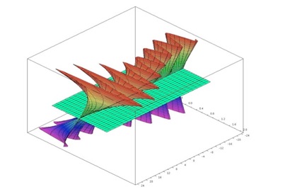
SIRS model: In order to investigate dynamical resonance in influenza epidemics, J. Dushoff, J.B. Plotkin, S.A. Levin and D.J.D. Earn (Dynamical resonance can account for seasonality of influenza epidemics, PNAS, 1-1, 16915-16916, 2004) study the following SIRS epidemic model
We choose parameters N=1, L=1, D=1 and the quasiperiodic driving functions β1(t)=1+sin(t)+sin(t/(3π)) and β2(t)=2.
The following graphic shows the saddle-point structure around the hyperbolic equilibrium (x,y)=(N,0). We obtained 5th order Taylor approximations of the corresponding time-dependent stable manifold (in green) and unstable manifold for t between -24 and 24. Both manifolds intersect along the t-axis.
In the subsequent illustration we have animated the quasiperiodic time-dependence of the above unstable manifold for t in the interval [-12,12].


Christian Pötzsche (Feb 2011)